LaTeX Lessons
Lesson One: Introduction
To download a LaTeX file in this lesson either copy and paste the latex code that follows into your editor
of choice, or alternatively you can copy the latex file into your directory by right-clicking the download link below,
and then select "Save Target As", followed by clicking on OK. If you like you can create a folder in your H: drive to
save this file e.g. H:\latex-lesson1\
\documentclass[12pt]{article}

\begin{document}

In here goes different styles of text, tables, arrays, pictures, etc. etc.

\end{document}
Download: latsam1.tex
Editing your LaTeX file
LaTeX files are plaintext files, so any text editor should be suitable for editing. Windows comes with a simple text editor called WordPad, but you can also use WinEdt, Tinn-r, TeXnicCenter, etc. Notepad, which also comes with Windows, can also be used but is not recommended if editing files created on a Unix/Linux system because of carriage-return differences.
Processing your LaTeX file
|
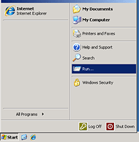
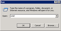
As you now have a LaTeX file in your directory, one still has to process it. Open a console (command prompt) by:
h:
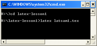
Note:all commands will be typed in the same console window (See Figure 1.3). To compile the document, enter the command: latex latsam1.tex
|
|
Processing information will appear on the window. Unless an error message appears, you can in general just ignore it. If there are errors, you will need to correct your document and re-run the latex command. If there are labeled items in your document (e.g. figures, table or equations), then you will need to run the latex command a second time.
Next the resulting .dvi file needs to be converted into a postscript .ps file with the command:
dvips latsam1
More processing information will appear which you can again ignore. Create a PDF from the LaTeX document by typing:
ps2pdf latsam1.ps
You can now view the PDF with the command:
start latsam1.pdf
A new window will appear which will show you the visual output of your LaTeX file which can be sent to the printers.
The steps to remember are:
latex the file:
latex file_name.texdvips the file:
dvips file_nameps2pdf the file:
ps2pdf file_name.ps
Notes:
- Spaces are ignored by LaTeX, see later lesson as to how to add spaces.
- Single carriage returns are ignored in LaTeX, double carriage returns are regarded as being a new
paragraph, to create a new line use either
\\or\newline. - Latex documents that include PDF images need to be compiled with the command
pdflatexinstead of thelatexcommand.
This concludes your first lesson on using LaTeX.
Lesson Two: Writing your First LaTeX File
LaTeX files are generally written by copying existing files and modifying to suit. As you already have the file latsam1.tex, open it in your text editor.
In this example, the file has been opened in WinEdt (see Figure 2.1). Alter the text in between the
\begin{document} and \end{document} using the mouse, arrow keys, and
backspace or delete keys. Example: alter the document to:
\documentclass[12pt]{article}

\begin{document}

Gosh I am now writing my first

LaTeX document.

\end{document}
Save the file by clicking on the icon with a picture of a floppy disk.
You will now need to LaTeX, and dvips as mentioned in lesson 1. You can save the file under a different name by clicking on the "File" menu and selecting "Save As".
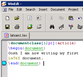
Figure 2.1 - WinEdt Window
There are macro buttons built in to WinEdt for calling the latex-related commands (see Figure 2.2). The "Latex" button is currently assigned to
the PDFLatex command, rather than latex command. Unless you are inserting images, in most cases this should
be fine. The DVI -> PDF button will convert the resulting .dvi file into a PDF file and then open it for viewing.
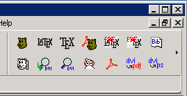
Figure 2.2 - WinEdt Window
This concludes lesson 2.
Lesson Three: Introduction to Fonts
Changing the size of the font
To change the size of the font, one must specify a size from the table below. For example with
the sample file shown below one can easily change the size of a font via the use of brackets
{} and \Large.
\documentclass[12pt]{article}

\begin{document}

{\Large Assignment 1}\\

To calculate the ...etc.

\end{document}
Download: latsam3a.tex
If you follow the procedure mentioned earlier of
- LaTeX the file via
latex file_name.tex - dvips the file via
dvips file_name - ps2pdf the file via
ps2pdf file_name.ps
You will see the effect of the \Large.
Edit the file, i.e.
xemacs latsam3a.tex &Now try out various different font sizes and re-latex and dvips them, making sure that you remember the brackets.
Notes:
- Not using brackets will just result in the document having that font from then on.
- You must use the brackets
{}not()or[].
| LaTeX | Output |
|---|---|
{\tiny Some Text} |  |
{\scriptsize Some Text} | |
{\footnotesize Some Text} | |
{\small Some Text} | |
Some Text | |
{\large Some Text} | |
{\Large Some Text} | |
{\LARGE Some Text} | |
{\huge Some Text} | |
Figure 3.1 - Various Font Sizes
Changing the style of the font
To change the style of the font, one must specify which style you wish from the table below, see example below.
\documentclass[12pt]{article}

\begin{document}

\noindent \textbf{Assignment 1}\\

To calculate the ...etc.

\end{document}
Download: latsam3b.tex
| LaTeX | Output |
|---|---|
Some Text |  |
\textit{SomeText} |  |
\textsl{SomeText} |  |
\textup{SomeText} |  |
\textrm{SomeText} |  |
\textsf{SomeText} |  |
\textbf{SomeText} |  |
\textsc{SomeText} |  |
\texttt{SomeText} |  |
Figure 3.2 - Various Font Styles
Combining different styles and sizes
One can combine font styles and font sizes together so that you can have for instance bold italics size large. See below for a working example.
\documentclass[12pt]{article}

\begin{document}

\textbf{{\Large O}nce more onto the breech dear \textit{friends}}

Let this be our summer of discontent

\end{document}
Download: latsam3c.tex

Figure 3.3 - Result of line 3 in previous code
This concludes lesson 3.
Lesson Four: Using Colour Fonts
Colour is mainly for presentations, keep in mind most of our printers are grey scale printers, and colour printing is expensive. But using greyscale within a paper or thesis can add aesthetics at no extra printing cost, but note photocopying may not come out the way you were expecting, so do test before running off 200 copies. As for sending as FAXs don't bother, some are set as black and white only.
Below gives a brief example on inserting standard colours.
\documentclass[12pt]{article}

\usepackage{pstcol}

\begin{document}

\noindent {\blue This is blue}\\

{\darkgray This is darkgray}\\

\end{document}
Download: latsam4a.tex
This is blue
This is darkgray
The following shows you a more extensive example on defining and inserting colours.
\documentclass[12pt]{article}

\usepackage{pstcol}

\newgray{darkergray}{0.3}

\newcmykcolor{tancmyk}{0 0.42 1 0}

\newrgbcolor{tanrgb}{0.98 0.67 0.33}

\usepackage{pstcol}

\begin{document}

\noindent \textcolor{darkergray}{This is darkergray}\\

\textcolor{tancmyk}{This is tan cymk}\\

\textcolor{tanrgb}{This is tan rgb}\\

\end{document}
Download: latsam4b.tex
This is darkergray
This is tan cymk
This is tan rgb
Try experimenting with defining colours of your own, see the Staff/Graduate guide to LaTeX for references to calculating rgb numbers.
This concludes lesson 4.
Lesson Five: Non-Standard Fonts
Included here are sample files containing each of the non-standard fonts mentioned in the School’s LaTeX guide. Please note that in some cases you may have to LaTeX twice before the fonts will appear in the document. Firstly the mathbb font without the curve. Note: font designed for uppercase.
\documentclass[12pt]{article}

\usepackage{amsfonts}

\begin{document}

$\mathbb{MOUSE}$

\end{document}
Download: latsam5a.tex
\documentclass[12pt]{article}

\usepackage{amsfonts}

\begin{document}

$\mathfrak{Assignment}$

\end{document}
Download: latsam5b.tex
\documentclass[12pt]{article}

\usepackage{amsfonts}

\newcommand\gothfamily{\usefont{U}{ygoth}{m}{n}}

\DeclareTextFontCommand{\textgoth}{\gothfamily}

\begin{document}

\textgoth{Assignment}

\end{document}
Download: latsam5c.tex
\documentclass[12pt]{article}

\usepackage{amsfonts}

\newcommand\frakfamily{\usefont{U}{yfrak}{m}{n}}

\DeclareTextFontCommand{\textfrak}{\frakfamily}

\begin{document}

\textfrak{Assignment}

\end{document}
Download: latsam5d.tex
\documentclass[12pt]{article}

\usepackage{amsfonts}

\newcommand\swabfamily{\usefont{U}{yswab}{m}{n}}

\DeclareTextFontCommand{\textswab}{\swabfamily}

\begin{document}

\textswab{Assignment}

\end{document}
Download: latsam5e.tex
This concludes lesson 5.
Lesson Six: Postscript Fonts
On the whole it is recommended that you stick with Mark Hickman's postscript font. But for those who which to create documents which are purely text i.e. no mathematics, then try experimenting with the 3 fonts Times (ptm), Helvetica (phv) and Courier (pcr).
For example (user defined variables in green):
\documentclass[12pt]{article}

\DeclareFixedFont{\MyFont}{T1}{pcr}{m}{n}{16pt}
This concludes lesson 6.
Lesson Seven: Creating an Itemised List
We will start with a simple example
\documentclass[12pt]{article}

\begin{document}

\begin{itemize}

\item One rope coloured red

\item One long bent thing with a lump on the end

\end{itemize}

\end{document}
Download: latsam7a.tex
This would produce the following list...
- One rope coloured red
- One long bent thing with a lump on the end
Next, an example showing nested itemisation
\documentclass[12pt]{article}

\begin{document}

\begin{itemize}

\item Wizard’s Equipment

\begin{itemize}

\item [$\Delta$] One rope coloured red

\item [$\Delta$] One long bent thing with a lump on the end

\end{itemize}

\item Warrior’s Equipment

\begin{itemize}

\item [$\dagger$] One big sharp pointy thing

\item [$\dagger$] One flat round thing

\end{itemize}

\end{itemize}

\end{document}
Download: latsam7b.tex
The above the example would produce the following output...
- Wizard’s Equipment
- One rope coloured red
- One long bent thing with a lump on the end
- Warrior’s Equipment
- One big sharp pointy thing
- One flat round thing
For browsers that do not support CSS1, the preceding example should look like this image.
This concludes lesson 7.
Lesson Eight: Creating an Enumerated List
Follow the example.
\documentclass[12pt]{article}

\begin{document}

\begin{enumerate}

\item This little pig went to market

\item This little pig stayed home

\end{enumerate}

\end{document}
Download: latsam8.tex
The results would be...
- This little piggy went to market
- This little piggy went home
End of lesson 8.
Lesson Nine: Writing Mathematics
Mathematics must always be enclosed within either two $ or between \( and
\), or between \[ and \] or between two $$, or
within an eqnarray or equation environment. To enclose text within mathematics you must use a
\mbox statement.
\documentclass[12pt]{article}

\begin{document}

When looking at $\alpha$ or $\beta^2$ one

frequently find that the coefficient

\( \chi-\frac{1}{2} \) results in

\[ \bar{x}=\sum_{i=1}^n x_i \]

$$ \frac{\partial y}{\partial x}=y $$

and with the equation

\begin{eqnarray}

\frac{\partial y}{\partial x} & = & \lambda

\end{eqnarray}

\begin{equation}

y=\frac{e^{-y/2}}{\sqrt{2*\pi}}

\end{equation}

\end{document}
Download: latsam9.tex
This would produce...
Figure 9.1 - Output from above example
End of lesson 9.
Lesson Ten: Creating an Array
We will start with the minimal array
\documentclass[12pt]{article}

\begin{document}

\[ \begin{array}{cc}

1 & 2 \\

3 & 4

\end{array} \]

\end{document}
Download: latsam10a.tex
The output is...
1 2
3 4
To insert a matrix into LaTeX, add the delimiters \left[ and \right].
For a full list of delimiters see a LaTeX manual.
\documentclass[12pt]{article}

\begin{document}

\[ \left[ \begin{array}{cc}

1 & 2 \\

3 & 4

\end{array} \right] \]

\end{document}
Download: latsam10b.tex
The output is...

You can also add lines around your array
\documentclass[12pt]{article}

\begin{document}

\[ \begin{array}{|c|c|}

\hline

\alpha^2-1 & \Delta \beta \\ \hline

\int x^2-x dx & \lim_{n}^{\infty} \frac{n^2}{n+1}\\ \hline

\end{array}\]

\end{document}
Download: latsam10c.tex
The output is...
This concludes lesson 10.
Lesson Eleven: Inserting EPS Figures
To import EPS (encapsulated postscript) figures into your document, the epsfig package is required. Insert command \usepackage{epsfig} after
the \documentclass definition:
\documentclass[12pt]{article}

\usepackage{epsfig}
Download: latsam11.tex and myfigure.eps
Inserting the EPS file
The basic code to insert an EPS format image into the document is as follows:
\begin{figure}

  \epsfig{file=myfigure.eps}

\end{figure}
Note: the above code has been indented. This is ignored by the latex compiler, but it useful to help people understand the code.
Images can be placed anywhere in the main document i.e. between the \begin{document} and \end{document}
tags. The latex compiler will place the image as close as possible to where the image is declared in the document, taking into
account other objects and page breaks.
Adding a caption the image
\begin{figure}

  \epsfig{file=myfigure.eps}

  \caption{This is a caption}

\end{figure}
Resizing the image
In the next example, the resizebox command has been used to set the size of the image:
\begin{figure}

  \resizebox{8cm}{!}{

    \epsfig{file=myfigure.eps}

  }

\end{figure}
Centering the image
The image can also be centered by inserting \begin{center} and \end{center} tags:
\begin{figure}

  \begin{center}

    \epsfig{file=myfigure.eps}

  \end{center}

\end{figure}
Putting it all together
\begin{figure}

  \begin{center}

    \resizebox{8cm}{!}{

      \epsfig{file=myfigure.eps}

    }

    \caption{This is a caption}

  \end{center}

\end{figure}
This concludes lesson 11.